Mechanistic Interpretability of Integer Addition in a 1-Layer Transformer

AISES Spring 2025 Project
Francisco Ferreira da Silva and Janice van Dam

Introduction

Artificial intelligence (AI) has advanced dramatically over the past decade, evolving from a specialized academic field into a significant force shaping global economics and geopolitics. Unlike traditional software which is directly programmed by humans, generative AI systems learn by training, resulting in capabilities that are often opaque. This lack of clarity regarding the functioning of AI models is a unique challenge in technological history and drives major concerns about potential misalignment, misuse, and reliability.

While slowing the rapid pace of AI development seems challenging, partly due to intense international competition, we can actively steer progress towards safer and more manageable systems. Improving the interpretability of AI is crucial to this effort. This report explores the vital field of mechanistic interpretability, which strives to reverse-engineer AI models, akin to developing precise neuroimaging for artificial minds, allowing us to understand, predict, and guide their behavior before their capabilities become overwhelming.

More specifically, we will look into a phenomenon referred to as grokking, first observed by Power et al. (2022) and further analyzed by Nanda et al. (2023). Grokking describes a surprising learning pattern where neural networks initially memorize training data (achieving high training accuracy but poor test accuracy), but then suddenly generalize to unseen examples after extended training, despite receiving no new information. This phenomenon offers a unique window into how neural networks transition from memorization to developing algorithmic understanding.

In “Progress Measures for Grokking via Mechanistic Interpretability,” Nanda et al. (2023) report on a comprehensive analysis of small transformers trained on modular addition tasks that exhibit grokking. They discovered that these models implement a sophisticated algorithm using discrete Fourier transforms to implement addition as rotations on a circle. Their analysis revealed that grokking is not a sudden shift but rather a continuous process with three distinct phases: memorization of training data, formation of generalizable circuits, and cleanup where memorization components are removed.

Building on this line of research, our work aims to test the generality of the grokking phenomenon and the mechanistic interpretability analysis techniques developed by Nanda et al. (2023) by shifting the focus from modular addition to the prediction of generalized Fibonacci sequences. In this task, we reverse-engineer how a small transformer learns to predict the next element, F(n), in the sequence given the two preceding elements, F(n-2) and F(n-1), where the sequences can begin with arbitrary starting values. This framing isolates standard integer addition, contrasting with the cyclical nature inherent to modular arithmetic. By investigating this task, we seek to explore potential differences in learned representations and algorithms for non-cyclical arithmetic within the transformer architecture. We aim to train the small transformer model in such a way that it exhibits grokking, followed by applying similar mechanistic interpretability techniques – including embedding, attention, and MLP analyses, as well as ablations – to gain insights into the learned mechanism. By addressing these questions, we hope to contribute to a more comprehensive understanding of how neural networks develop generalizable algorithms and how we might predict and interpret emergent behaviors in more complex models.

Setup

The transformer used here is exactly the same as that described by Nanda et al. (2023): a one-layer ReLU transformer, token embeddings with dimension 128, learned positional embeddings, 4 attention heads of dimension d/4 = 32, and 512 hidden units in the multilayer perceptron (MLP). The model is trained using an AdamW optimizer with a learning rate of 1E-3 and a weight decay of 1.

In addition to defining the model, we define a dataset describing the Fibonacci problem – which equals regular addition. The input data is any set of two integers between 0 and N, plus a special ‘equal sign’ token, described by the number N. The labels, i.e., the expected outcome, is the sum of the two integers, which is between 0 and 2N. Each number is encoded as an N-dimensional one-hot vector.

A fraction df of the full dataset is used to train the transformer. The model is then tested on both the training set, as well as the remaining set of inputs the model was not trained on, the test set. To observe grokking, the input space size N and the training fraction df need to be carefully controlled such that the training set size is small enough to make it easy for the model to learn the outcomes initially by memorization, but large enough such that the model will eventually be able to generalize to the test set.

We found that for N=10, and thus an input space of 100, and a data fraction of 0.72, we observe grokking in the model, as shown in Figure 1.

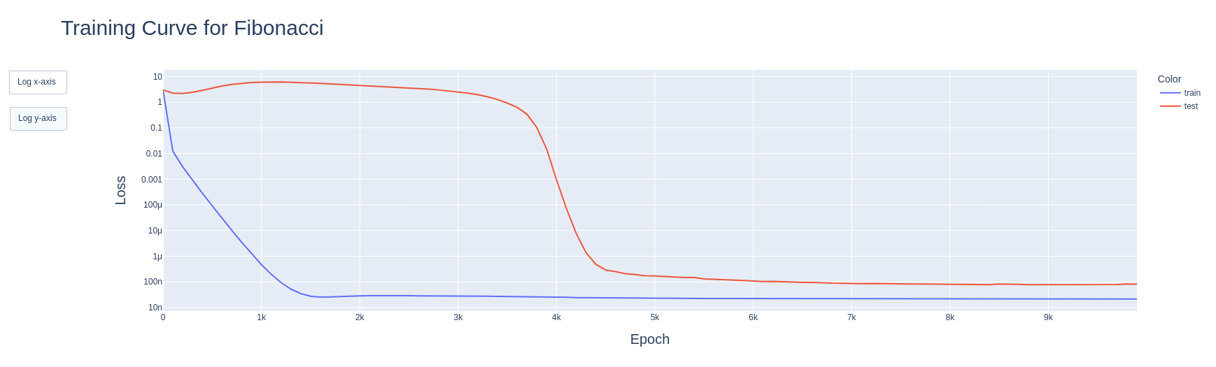Figure 1: Observing grokking. First, the training loss goes down quickly, indicating memorization. Later the test loss also quickly falls, indicating the model having found a generalizing algorithm to solve the problem.

Results

The central question of this investigation is: what algorithm did the transformer learn to solve the generalized Fibonacci (i.e., standard integer addition) problem? We applied several mechanistic interpretability techniques to dissect the trained model.

As a first step, we analyzed the learned token embeddings, WE, for inputs 0 through 9 using Principal Component Analysis (PCA). The first principal component (PC1), accounting for approximately 73% of the variance, showed a linear correlation with the input token value. The second principal component (PC2), explaining an additional ~26.4% of the variance (totaling ~99.4% for PC1+PC2), had a quadratic relationship with the input token value. This indicates that the model learns to represent the numerical inputs primarily using features corresponding to their linear value and a quadratic component, sensitive to the input’s position relative to the range boundaries.

One would expect that a linear component would be enough, as addition is a linear operation. Hence, we performed an ablation study in which we removed the quadratic feature (PC2) from the learned embeddings before passing it along to the rest of the transformer. This caused a drop in test accuracy from 100% to approximately 40%, indicating that whatever algorithm the network has learned, it definitely depends on this quadratic feature.

Analyzing the specific errors made by the PC2-ablated model revealed systematic failure patterns, as shown in the figure below where we plot the prediction error (i.e., the difference between the prediction of the ablated model and the true sum). The ablated model appears to struggle at the boundaries (when either one of the inputs is 0 or 9, although surprisingly not when both are) and when they are roughly symmetric, as well as with values close to the mean of the possible input space.

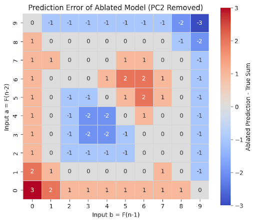Figure 2: Prediction error of the ablated model. It appears to struggle at the boundaries (for inputs close to 0 or 9, although interestingly not if one of the inputs is 0 and the other 9), and for roughly symmetric input values.

Another ablation study we performed was to remove the skip connection around the MLP. This resulted in negligible changes to model performance, measured by both accuracy and loss, indicating that the model’s output can reliably be approximated by multiplying the unembedding matrix with the output of the MLP.

With this in mind, we focused on understanding the computation performed by the MLP. We observed that both the pre- and post-ReLU states were well-modelled by a quadratic polynomial of the principal components (note that this means quartic in the original inputs, as the second principal component is itself quadratic on the inputs). Further, we observed that restricting the quadratic models that we fit to be symmetric with respect to a and b (or, alternatively, to depend only on their sum) decreased fit quality only very slightly, indicating that the MLP indeed treats both inputs symmetrically.

This quadratic relationship held with high fidelity across the majority of the 512 neurons in the MLP layer (mean R² > 0.998 pre-ReLU, mean R² ≈ 0.975 post-ReLU when fit against the polynomial features of the principal components). This suggests a highly distributed computation.

However, analyzing the readout step performed by the unembedding matrix WL revealed a contrast. PCA performed on the columns of WL (where each column represents a neuron’s influence on all output logits) showed that the structure of this readout matrix is low-dimensional. The first two principal components alone captured over 98% of the variance in how neurons map to output logits. This indicates that while hundreds of neurons compute features based on the input PCs, the final output is constructed by projecting these activations onto a very simple, shared 2-dimensional basis embedded within WL. Therefore, despite the broad participation of neurons in the MLP, the information relevant for the final logit calculation is compressed into a very low-dimensional subspace by the learned unembedding weights, indicating redundancy in the MLP representation stage.

Ultimately, the network converges on an algorithm where the final logit for each potential sum k is equivalent to a quartic polynomial of the original inputs a and b (quadratic on the principal components), as shown in the plot below for the inputs (0,0).

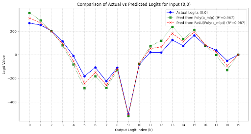Figure 3: The blue line corresponds to the actual logits of the transformer for inputs (0,0). Note that they peak at 0, as expected. The green line corresponds to replacing the output of the MLP layer by a quadratic fit to the principal components. The red line is the same, but the fit is done just before the ReLU.

Along the same lines, we also fit the logits for each possible input pair to a quadratic function of the principal components and obtained R²>0.95 for all fits.

Discussion

The results found are somewhat unsatisfying. Whereas Nanda et al found that their model learned a very simple, elegant algorithm for modular addition, ours converged to a very convoluted one — learning complex quartic polynomials to implement a simple linear function. We note that for the simple task we defined, the model could have simply passed the inputs along via the skip connection, even obviating the need for the attention heads and the MLP. It is in one sense interesting that it does not do this and does seem to make use of its transformer features, but it is on the other hand slightly frustrating that it converges on such a complex algorithm.

Although theorizing about why models learn something is murky territory, let us try. The input space we defined was very small (only 100 unique input pairs), especially in comparison with the size of the model (128-dimensional embeddings, four attention heads, 512 neurons in the MLP). This means that there is a lot of redundancy, and hence many possible pathways for the model to learn how to implement the sum. In that sense, considering a more challenging problem, using a larger input space, or scaling down the model size could all have encouraged the model to learn a simpler, more elegant algorithm.

This brings us to possible directions to extend this work. As mentioned, one possibility is to increase the size of the input space. We note that this would necessarily bring us into the realm of multi-digit addition, which is inherently more complex: for example, the model needs to learn to perform carries, and it would be interesting to see if specialized circuits for this operation would arise.

Going back to the original motivation of this work, which was to study sequences, in particular the Fibonacci sequence. The way in which we defined the input space resulted in the task of predicting the next element in the Fibonacci sequence effectively becoming equivalent to addition. We could generalize this by allowing for inputs of variable length, i.e., having some inputs with two elements of the sequence, some with three, etc., with the desired output remaining the following element.

From an AI safety perspective, this work illustrates the challenges of understanding learned AI behavior. We found that the model learned a complex solution for a simple task, which was a priori not to be expected from its input-output behavior. It is also humbling to realize how much work went into painting this picture, given how simple the model and the task are in comparison with the state-of-the-art models and practically useful tasks.

References

Nanda, Neel, et al. “Progress measures for grokking via mechanistic interpretability.” arXiv preprint arXiv:2301.05217 (2023).

Power, Alethea, et al. “Grokking: Generalization beyond overfitting on small algorithmic datasets.” arXiv preprint arXiv:2201.02177 (2022).

Code Availability

The Jupyter notebook used to run all experiments on which we report here can be found at https://github.com/FranciscoHS/ai-safety-project-2025.

Author Contributions

Francisco and Janice co-designed the project and ran most of the experiments together. The initial draft of the report was made by Janice, with the final version mostly being written by Francisco.